
Definition of Engine Belt length Using the Statistic Dimensional Variation Analysis and Assembly Variation of Front Engine Accessories Drive
David Santos Baião
Cummins Brasil Ltda
Dennis Alberto Baião
Célere Engenharia e Treinamentos Ltda ME
Dan Lange
Sigmetrix, LLC
ABSTRACT
This is a solid methodology to define and/or verify how the dimensional schema of the parts and their statistical variation affect the assembly variation.
This study has been done to fix an issue in the assembly line of a Cummins’ customer. This is a problem that occurs during the assembly of the Linear Belt Tensioner.
The voice of customer says “Many times it is too hard to assemble the Belt Tensioner!”
The paper shows the analysis performed at Cummins Brazil. The analysis process utilized the Dimensional Variation Analysis methodology, statistical software – Minitab, Pro/Engineer and CETOL 6σ to verify the length of the FEAD (Front Engine Drive Accessories) belt path. , the results were compared with the variation of the Belt length.
The voice of customer was proved by the three-dimensional DVA analysis. The design shows up to 16% of the FEADs could have problems during the assembly. The improvement in the assembly line and in the design has been defined based on these results and methodology.
INTRODUCTION
History of Dimensional Variation Analysis
The Dimensional Variation Analysis (DVA) has evolved along with quality methodologies applied in the factories, especially in the automobilist industry. Nowadays, it is possible to predict how variation will affect product yield.
During the 1930’s, Walter Shewhart introduced some basic concepts in factories including statistics and scientific methodology in the United States. He was the pioneer of Statistical Process Control (SPC) in the manufactory process.
Nowadays, there is no factory in the world which does not apply at least some basic tools of SPC for processes improvements.
Over the years, quality and manufacturing technology has improved. Standard tolerances have been defined and included in the International Organization for Standardization (ISO) and adopted by standards like NBR 6158, asme_Y14_5M_2009 and others. However, this standard only describes how to use and interpret the tolerances for two features, one that is a hole and the other is a shaft.
According to Stanley Parker (creator of GD&T) the Classical Dimensioning & Tolerancing or in other words, the Cartesian System, should be applied in only a single item: the tolerance on nominal dimensions, because this system is totally unable to define coordinate systems. To solve this problem Stanley Parker created another method to specify tolerances called GD&T (Geometric Dimensioning and Tolerancing), that is more capable of defining design intention. While GD&T can be very useful in defining design intent and part acceptance guidelines, the actual process variation must still be analyzed in order to consistently and cost effectively build high quality assemblies.
If we look at a stack up of parts we can calculate the worst case by summing the tolerances of related parts.
Manufacturing processes are rarely uniform and within an assembly, several distribution types may be presents. The most common distribution is called Normal. The results are very different between these methodologies.
In the real world the worst case is not true, in fact if the parts are under of the normal process the probability to find an assembly in the maximum condition or minimum condition is quite impossible. By other hand, the assemblies could be of different distribution types and it is necessary to use another technique to get an accurate result.
Purpose of Dimensional Variation Analysis
The purpose of Dimensional Variation Analysis is to achieve a robust design recipe while also arriving at a “thoughtful allocation of economic tolerances”. The process is best employed early in the Design/Development process when it is still possible to change nominal geometry in order to desensitize the design to variation. Dimensional Variation Analysis methods are revisited in final preparations for production release and also employed for making later product changes for cost improvements or correcting reliability issues. Figure 2 – The value of DVA and early, proactive, concurrent engineering illustrates the importance of performing the appropriate DVA activities early in the design cycle in order to achieve the future goal of optimum concurrent engineering leading to more rapid release of robust production designs.

Benefits of Dimensional Variation Analysis
A. Achieves robust design with managed low risk of failure (low warrantee cost);
B. Achieves thoughtful allocation of economic tolerances for reduced manufacturing costs;
C. Allows Design Engineer greater flexibility in achieving design targets with comparative advantage;
D. Focuses quality efforts on only the necessary, critical tolerances (saves inspection); and
E. Enables improved, data-based concurrent engineering and communication between design, development, manufacturing, purchasing, suppliers and quality.
Defining the Dimensional Variation Analysis objective
This is the most crucial step in the process and it is important to be specific in defining the objective. For example, one might want the clearance between the Ø70mm on the piston skirt to the ID of the liner bore, or the angular alignment of two specific pulleys, or the minimum wall thickness at location X after machining, or the gasket sealing surface from the R12 on the gasket to the R15 on the head. In other words, it is necessary to be more detailed in the description of the DVA objective that simply stating a generic objective such as “filter to bracket clearance”.
Identify all components involved in the Dimensional Variation Analysis
After the DVA objective is set, one can typically determine what components are required to determine that objective. The “correct” revision of the drawing should be pulled. For most cases one would want the latest revision of the drawing, however, if one is involved in a field failure one needs the drawing revision used at the time the assembly was produced.
Most Design Engineers would intuitively make a sketch of their assembly to enable them to picture what the DVA objective is, determine what the dimensional loop is, and identify the relevant features of the individual components.
There are many tolerances and dimensions on engineering drawings that can become overwhelming and confusing. Identify the relevant dimensions, tolerances and datums on the drawings.
Loop Method Loop method is a standard, rigorous, and yet simple process whereby the userdevelops the mathematical model required to describe the system or relationship in question. The loop method forces the user to identify all necessary components (and their tolerances) in the “loop” by systematically marching through the assembly from the start point to the end point of the relationship to be analyzed. The Figure 3 – The Loop Method and Figure 4 –Simple Example of the Loop summarizes the loop method using an example involving three blocks and evaluation of the internal gap between two of the blocks. Note that the start and end point could be interchanged and the sign convention used (positive from right to left) could be chosen alternately, based on the user’s preference. It is recommended, however, that the positive direction coincide with the direction from start point to finish point in order that resulting clearance values make intuitive sense. Positive value denotes clearance and negative value denotes interference.

Statistical Variation Analysis
The statistical variation analysis model takes advantage of the principles of statistics to relax the component tolerances without sacrificing quality. Each component’s variation is modeled as a statistical distribution (Figure 5 – Statistical stack up variation) and these distributions are summed to predict the distribution of the assembly measurement. Thus, statistical variation analysis predicts a distribution that describes the assembly variation, not the extreme values of that variation. This analysis model provides increased design flexibility by allowing the designer to design to any quality level, not just 100 percent.

Many engineers are familiar with basic statistical stack up methods, such as RSS (Root Summed Squares) analysis. RSS uses a number of simplifying assumptions that are too restrictive for a full-featured statistical variation analysis tool. Use a more general statistical technique called the Method of System Moments. This method works directly with the statistical distributions of each part variable to calculate the distribution for the stack up measurement. Using this method, the software CETOL 6σ can include non-linear geometric behavior and non-normal variable distributions when calculating the measurement variation.
Distribution Types
There are many ways of representing a population statistically that can be defined in terms of three distribution types: normal, uniform, and SMLambda (Standard Moments Lambda) distributions.
A normal distribution (Figure 6 – Normal distribution) can be completely defined in terms of two parameters: mean and standard deviation. It is easily transformed to scaled moments for analysis purposes. The skewness of a normal distribution is 0.0, and the kurtosis is 3.0. A normal distribution has infinite tails.

A uniform distribution (Figure 7 – Uniform distribution) can be completely defined in terms of two parameters: min and max. These parameters can be transformed to scaled moments for analysis purposes. The skewness of a uniform distribution is 0.0, and the kurtosis is 1.8.

The lambda distribution is a statistical distribution defined in terms of four lambda parameters. The Standard Moments Lambda (SMLambda)distribution (Figure 8 – SMLambda distribution) is a very flexible generic distribution defined in terms of four lambda parameters: mean, standard deviation, skewness and kurtosis. The values for skewness and kurtosis must be within certain limits in order fit a SMLambda.

MODIFIED RSS (MRSS) STATISTICAL ANALYSIS
Tier Modified RSS represents the introduction of the phenomenon of compound probability distributions and statistics into Dimensional Variation Analysis. In a high volume manufacturing setting, the compound probability that all contributing tolerances in a given variation analysis problem will be at the extreme print limit is extremely remote. Therefore the total amount of variation the product will experience in production will only be a fraction of the magnitude of the Worst Case results. For this reason, consistently designing products to Worst Case results will compromise comparative advantage by creating products that will be unnecessarily large, heavy, and costly.
The most common method used in the past to simulate the effects of compound probability is the Root Sum Squared (RSS) technique. The total statistical variation resulting from a list of additive, independent, nominal-centered, and Gaussian (normal) distributions is given by RSS in the following formula Equation 1– RSS formula:

Where Tn is the individual tolerance. The weakness of the RSS technique has to do with the assumption that all distributions are perfectly nominal-centered and perfectly Gaussian, or normal. While these two assumptions allow for a simple calculation of compound probability, they do not represent the vast majority of manufacturing processes and quality control systems which exist in the real-world production environment. In fact, many manufacturing processes intentionally target values to one side of the print nominal in order to allow for greater tool wear and therefore tool life. Other quality control systems rely on inspection processes to screen “out-of-spec” parts yielding distributions which do not resemble Gaussian. For these reasons the RSS method yields results which may significantly underestimate actual production variations. Designing products using the RSS method will compromise market share by allowing the release of products with little or no design margin which will result in costly reliability and field failure issues.
As the number of tolerances in a particular analysis increases, the error resulting from the Worst Case and RSS methods also increases, as seen in Figure 9 – Worst Case vs. MRSS vs. RSS. The Worst Case curve is significantly larger and more conservative than the reality curve while the RSS curve grossly under-estimates reality. Therefore an analytical solution yielding an accurate, intermediate value is required to simulate reality, which will be referred to hereafter as the Modified Root Sum Squared or MRSS analysis.

Monte Carlo Simulation
Another technique to define the statistical variation of an assembly is to simulate the values using Monte Carlo analysis using statistical software (e.g. Minitab).
The below table shows the comparative analysis between Worst Case, RSS, MRSS and Monte Carlo using the example of Figure 4 –Simple Example of the Loop.
In the case 1 all dimensional inputs were left as normal distribution and in the Case 2, the dimension value 60 was changed for uniform distribution.

REAL CASE: Difficulties to Assembly the Belt in the Engine Cummins ISBe in the FORD Assembly Line – Voice of the Customer (FORD)
 “It is difficult to assemble the belt in some Cummins engines ISBe 4 and 6 Cylinders with the linear belt tensioner, and with or without the air conditioner”.
“We believe that the variation of position of the front engine arrangements drive (Figure 11 – Cummins Engine ISBe – Front Engine Arrangements Drive) is providing a too much variation in the FEAD (Front Engine Arrangements Drive) length”.
As informed by FORD the belts used in the FEAD of Cummins Engine ISBe 4 and 6 have the length 2063±5mm for application with Air Compressor and 1515±5mm for applications without Air Compressor, and the Belt Tensioner is compressed by the device with a size of 133.5mm shown.

FORD ASSEMBLY PROCESS
The components Damper Pulley, Water Pump Pulley, Idler Pulley and Air Compressor are fixed in their position but the alternator is not fixed in the linear , in fact the is not assembled in the engine.
A worker assembles the belt in the FEAD pulleys (Alternator, Damper, Water Pump, Idler and Compressor Air), but the Belt is not tensioned because the Alternator is not assembled yet (Figure 13 – Cummins ISBe Front Engine Arrangements Drive with Alternator not assembled at the Tensioner Belt ).
 Another worker compresses the Belt Tensioner in a special device to a specific dimension (123mm) and he assembles it at the Water Connection and at the Alternator housing (Figure 14 – Cummins ISBe Front Engine Arrangements Drive with Alternator assembled at the Tensioner Belt), so the device is removed and the Tensioner released and it apply tension to the belt.
VARIATION IN THE POSITIONS OF FEAD
The variation in the position of arrangements is based on the fixing method (parts only fixed with bolts have more position variation) and the variation in the assembly will be explained using the numbers shown in the Figure 15 – Variation in the FEAD position.
Arrangements:
1. Damper pulley has low variation because it is centered with the Crankshaft;
2. Idler pulley has high variations in the Y and X orientation in order to be assembled in the front face of block by 2 bolts;
3. Head Cylinder has medium variation in the Y orientation because there is a gasket between it and the block, the variation in X and Z is very low.
4. Alternator and air compressor support has high Y and Z variation according to be only fixed by screws, the X variation is low;
5. Air Compressor has low X, Y, and Z variation according the drawing tolerances;
6. Alternator has high X, Y and Z variation according the assembly system;
7. Water connection has high variations in the Y and Z orientation in order to be fixed by 3 bolts;
The variation of the Belt Tensioner is not mentioned because it is a flexible part and its deviation is part of the result of this paper.
 FEAD LENGTH
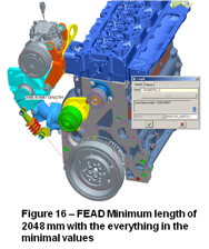
The length of the FEAD is based on the position of the components and mainly in the Belt Tensioner measurement lengthwise, the nominal end the minimum FEAD length is showed in the REF _Ref292377152 \h Figure 16 – FEAD Minimum length of 2048 mm with the everything in the minimal values and Figure 17 – FEAD Nominal length of 2062 mm with the everything in the minimal values, the values only consider the nominal position and dimensions of every arrangement.
ASSEMBLING THE LEAD IN THE SOFTWARE CETOL 6σ
“CETOL 6σ is the premier tolerance optimization technology in the world. The software accommodates a number of tolerance management needs through its unique dimensional analysis system that is engineered to support robust product development processes from design through manufacture. Unlike any other tool in the industry, CETOL 6σ is built on 3D Variation Behavior Modeling™ Technology and is fully-integrated with Pro/ENGINEER, CATIA V5, and SolidWorks – allowing for precise sensitivity, statistical and worst case scenario tolerance analysis” (Sigmetrix web site – https://www.sigmetrix.com/.
This analysis has been done using the CETOL 6σ ver 8.2 and Pro/ENGINEER Wildfire 4, to perform the analysis it is required to have an assembly with all involved parts.
First Step: The connection
First it is necessary to have an assembly file open in Pro/ENGINEER and make a link between CETOL 6 Sigma and Pro/E (Pro/engineer) as shown in the Error! Reference source not found., then create the assembly features in CETOL 6 Sigma
Second step: Add the assembly features in the CETOL 6σ
CETOL 6σ allows you to add an assembly overlay in which you define the assembly constraints with kinematic joints. CETOL’s kinematic joints allow you to very precisely represent the physical constrains of the assembly and also allow you to introduce the effects of assembly-level variation.
The assembly in the CETOL 6σ is created by Joints. Joints are used to define the constraints between the features of two components in the assembly.
When you create a joint, CETOL 6σ automatically determines the contact region between the selected geometry. The default joint attachment points on each part are at the center of the contact region (Figure 19 – Joint Properties). CETOL 6σ defines a connection between the attachment points on each part and applies the constraints at those points.
In the Table 1: Front Engine Arrangement Drive assembled at CETOL 6σ is shown the assembly scheme of each arrangement. The Figure 31 – Cummins ISBe FEAD assembly diagram in the CETOL 6σ (Assembly level) in the appendix shows the CETOL Model Graph.

When you create a joint, the DOF (degree of freedom) state for the joint is automatically set based on the selected features. The DOF editor shows a triad that represents the joint coordinate system. This triad corresponds to the triad that is displayed in the CAD system when the joint is selected. There is a translational and a rotational DOF associated with each joint axis. Each DOF can be either constrained or unconstrained.
The Bias setting allows you to specify the bias condition for some joint types. For example, for a pin in a hole you can specify the pin to be centered in or tangent to the hole. When you change the bias setting for a joint, the joint symbol in the CAD model updates to indicate the joint location.
FEAD Assembly Scheme
Every part of FEAD has its own assembly scheme and its own variation

Components dimensional Schema
In CETOL 6σ, it is possible to add the GD&T of all related parts and use these tolerances to perform the analysis of variation.
The schema will be shown in CETOL 6σ as a Part Network Diagram with the GD&T with the reference datums. In the Figure 20 – Dimensional Scheme in the CETOL 6σ is shown a small part of the dimensional schema of the alternator support.

To perform the analysis required the creation of the dimensional schema for every related part, but only dimensions and GD&T related to the features used to assembly modeling.
Result Analysis of Arrangements Position Variation
CETOL 6σ cannot calculate the variation of FEAD length directly but with CETOL it is possible to perform the analysis of the position variation of every arrangement.
The position variation has been performed to verify the deviation in the direction X and Y for the pulleys positions of the Alternator, Water Pump, Freon Compressor and Idle Pulley, using the crankshaft as the primary orientation.

The variation is showed as a Statistical Variation Plot and this plot shows a graphical representation of the statistical distribution of the every X and every Y measurement. The Figure 22 – Measurement Statistical Variation Plot shows an example of the Statistical Variation Plot.

The measurement specification limits and the target value are user specified values. These define the design requirements for the measurement. The assembly variation for each measurement is represented by a statistical distribution.
Using a CPK of 1.5 the lower and the upper engineering measurement limits for X and Y position of the pulley have been defined.
BELT DEVIATION LENGTH USING THE PRO/ENGINEER
“Pro/Engineer is the standard in 3D product design, featuring state-of-the-art productivity tools that promote best practices in design while ensuring compliance with your industry and company standards. Integrated, parametric, 3D CAD/CAM/CAE solutions allow you to design faster than ever, while maximizing innovation and quality to ultimately create exceptional products” http://www.ptc.com/product/creo/3d-cad/parametric/extension/tolerance-analysis.
Based on the mean of the dimension X, the dimension Y and the diameters of the pulleys, a sketch of the belt has been created in the Pro/Engineer.
Based on the lower and upper engineering limit the Monte Carlo method has been used to generate 4,000 interactions for each X and each Y pulley position. The data dimensions have been inserted into the Multi-Objective Design Study tool from Pro/Engineer to perform the FEAD length variation (Figure 23 – FEAD length calculated by Pro/Engineer 4.0).
The Multi-Objective Design Study is used to randomize all the X and Y dimensions in the sketch, regenerate the sketch, and measure the length of the lines. Pro/E shows the results in a table which can be saved in a data file to be studied in other software.
ANALYZING THE DATA IN THE MINITAB VER.15
“Minitab is the leading provider of software for statistics education and Lean, Six Sigma, and quality improvement projects. For nearly 40 years we have been helping world-class organizations analyze problems, transform their business, and train their students” (http://www.minitab.com/en-US/default.aspx).
The first step in the Minitab is: Verify if the data from belt length follows a normal distribution. To verify it is necessary to generate a normal probability plot and performs a hypothesis test to examine whether or not the observations follow a normal distribution. For the normality test, the hypotheses are, H0: data follow a normal distribution vs. H1: data do not follow a normal distribution.
The Anderson-Darling test’s p-value indicates that, at a levels greater than 0.05, there is evidence that the data do not follow a normal distribution (hypothesis Ho).
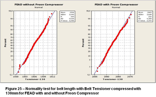
As the Figure 24 – Normality test for belt length with Belt Tensioner compressed with 117mm, 123mm for FEAD with and without Freon Compressor and Figure 25 – Normality test for belt length with Belt Tensioner compressed with 130mm for FEAD with and without Freon Compressor show the lengths variation created by Pro/Engineer the P-value for belt Tensioner compressed at 117mm is 0.118 and 0.480 for compressed at 123mm is 0,117 and 5.03, than the data follows normal distributions for the four cases. The p-value for Tensioner belt at 130mm is 0.372 and 0.096, than all data result follows the normal distribution.

As the data follows a normal distribution it is possible to have the length Mean, Variation and the lower and Upper limit to have the CPK of 1.33 (process capability of 1.33).
CPK is a measure of potential process capability calculated with data from the subgroups in your study. This represents the distance between the process average and the specification limits, compared to the process spread.
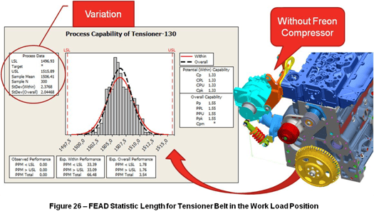
According to the work length of the Tensioner belt (130mm) the length of the FEAD without Freon compressor has a mean of 1506.41mm and a standard deviation of 2.3768 mm (Figure 26 – FEAD Statistic Length for Tensioner Belt in the Work Load Position).
VALIDATING THE VOICE OF THE CUSTOMER
According to the voice of customer says “It is difficult to assemble the Belt in some engines Cummins ISBe 4 and 6 Cylinders with Linear Belt Tensioner with and without Air Conditioner”. To analyze this problem further more information was received from the FORD assembly process and components.
As informed by FORD the belts used in the FEAD of Cummins Engine ISBe 4 and 6 have the length 2063±5mm for application with Air Compressor and 1515±5mm for applications without Air Compressor, and the Belt Tensioner is compressed by the device with a size of 133.5mm as the Error! Reference source not found.shows.
Using the size of the Belt Tensioner is possible to construct a FEAD length to compare with be belt length. To avoid troubles in the assembly process of the Belt at the FEAD, the length of the Belt has to be greater than the FEAD length otherwise the assembly process will be difficult.
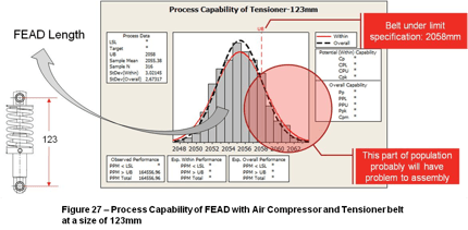
The Figure 27 – Process Capability of FEAD with Air Compressor and Tensioner belt at a size of 123mm shows the process capability of FEAD with Freon compressor using the Tensioner belt with 123mm (center hole to center hole) of size for a belt at the lower limit specification (2058mm). According to the PPM UB approximate 16% of the engines will be difficult to assembly.
P.S. There is no information about the distribution of the Belt length, so the worst case for the under length limit has been considered in the analysis.
The Figure 28 – Process Capability of FEAD without Air Compressor and Tensioner belt at a size of 123mm shows the process capability of FEAD without Freon compressor using the Tensioner belt with 123mm (center hole to center hole) of size for a belt at the lower limit specification (1510mm). According to the PPM UB approximate 0% of the engines will be hard to assembly.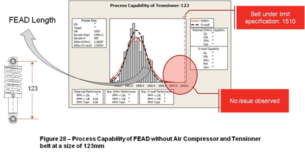
SUMMARY/CONCLUSIONS
SOLUTIONS FOR FEAD WITH FREON COMPRESSOR
To solve the issue with the FEAD with Freon Compressor there are two solutions that can be applied.
Solution #1: Change of the amount the Belt Tensioner is compressed in the assembly process.
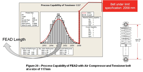
If the Tensioner Belt size changes from 123mm to 117mm (mechanical limit of the Tensioner Belt) the FEAD length will decrease enough to assemble the Belt without problems (PPM UB approximate 0%) as the Figure 29 – Process Capability of FEAD with Air Compressor and Tensioner belt at a size of 117mm shows.
 This change was required in the assembly device to achieve the design requirement.
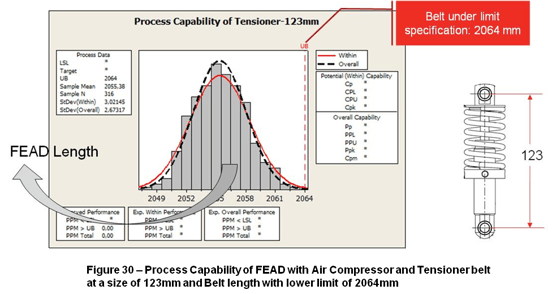
Solution #2: Increase the lower limit of Belt Length to 2064mm
If the lower limit of Belt length changes from 2058mm to 2064mm (New Belt) the FEAD length will be smaller enough to assembly the Belt without problems (PPM UB approximate 0%) as the Figure 30 – Process Capability of FEAD with Air Compressor and Tensioner belt at a size of 123mm and Belt length with lower limit of 2064mm shows.
This change requires FORD to develop a new Belt for this FEAD.
P.S. According to information from customer FORD, solution #2: Change the amount the Belt Tensioner is compressed in the assembly process has been implemented in the production process and no issues have been occurred.
The employees have been trained to use the changed device and how assembly correctly the belt in the FEAD.
REFERENCES
1. User Reference Manual of CETOL Version 8.2 for Pro/ENGINEER
2. Basic Training Manual of CETOL Version 8.1 for Pro/ENGINEER
3. Help of Minitab® 15.1.30.0.
4. Cummins Six Sigma Belt Training Material